Baseline Noise: Root Mean Squared (RMS) Noise Calculations - Tip297

OBJECTIVE or GOAL

Use root mean squared (RMS) noise calculations. 

ENVIRONMENT

• Empower
• Empower Tip of the Week #297

PROCEDURE

RMS calculations yield significantly smaller noise calculations, at least two-thirds smaller than equivalent peak-to-peak calculations. When working with drifting baselines or baselines with infrequent noisy regions, averaging segments of time over the measured noise region can give smaller calculated noise numbers. 

STEP 1
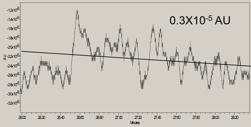
With an RMS noise calculation, we fit the noise to a best fit line using the linear least squares method (Figure 1).

STEP 2
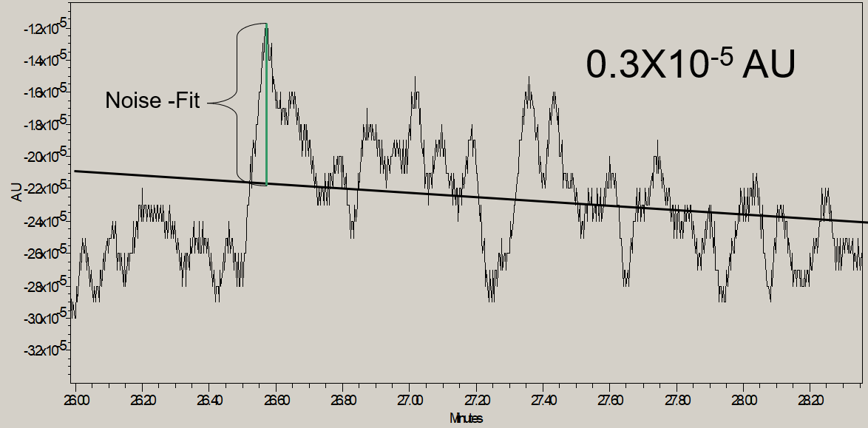
The difference between each noise point is subtracted from its corresponding calculated point on the best fit line. These values are summed, squared, and then averaged. The square root of this average value is reported as the noise in the RMS calculation (Figure 2). 

STEP 3
The noise is measured as distance from the best fit line. The noise region comprises parallel lines with the same slope as the original best fit line. Because this noise is measured with a best fit line following the slope of the baseline, the calculation is not dramatically impacted by a sloping baseline (Figure 3).

STEP 4
Even though the calculation is not dramatically impacted by baseline slope, the calculation may be broken into segments and averaged like the peak-to-peak calculation discussed in Tip #295. By doing this, you can average out the impact of outliers in the noise calculation (Figure 4).

STEP 5
If you break the noise region into thirty-second segments as before, you can do the linear least squares fit over each thirty-second segment (Figure 5). 

STEP 6
The noise is calculated for each segment, and the software arrives at a final, single number derived from these segments (Figure 6).

 

ADDITIONAL INFORMATION

This can be done with either the Pro or QuickStart interface.