Exploring calibration curve parameters within the processing method that can affect the calculation of amount or concentration - Tip269

OBJECTIVE or GOAL

This article explores calibration curve parameters within the processing method that can affect the calculation of amount or concentration, such as Average By and Fit. 

ENVIRONMENT

• Empower
• Empower Tip of the Week  #269 

PROCEDURE

AVERAGE BY: this function instructs Empower how to average the response of standard injections. The averaged response will be used to plot the calibration curve.

STEP 1
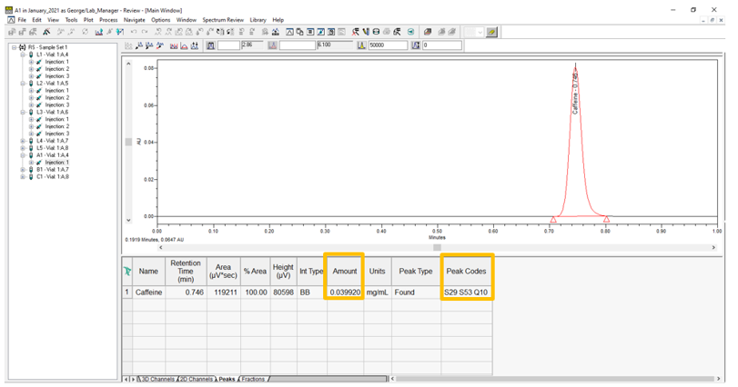
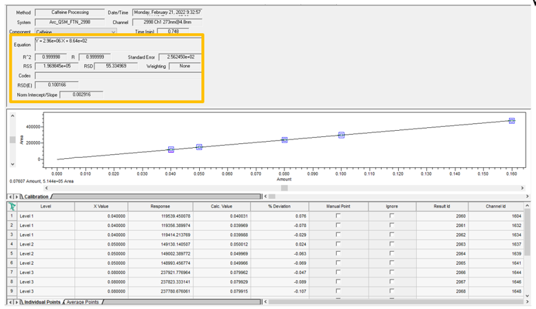
With the ‘Average By’ set to ‘None’ (which is the default), no averaging of standard injections takes place. In this example, we have three injections of each standard, and remember from the previous tips, each standard has a different amount of analyte. The equation, R, R2 and so forth can be seen in the calibration window within Review (figure 1).

STEP 2
The amount of Caffeine is reported as 0.039920 mg/ml. The Q10 Peak Code indicates that the response of the peak in the sample is lower than the response of the peak in the standard with the lowest amount (figure 2). 

STEP 3
Selecting ‘Average By, Amount’ will result in an averaged response calculated for the replicate injections at each amount (figure 3).

STEP 4
The calibration curve is plotted as ‘Amount’ versus ‘Averaged Response’. Note that the R, R2 and so forth have slightly different values (figure 4). 

STEP 5
The calibration curve is close to the original calibration curve resulting in a calculated amount of caffeine of 0.039920 mg/ml, essentially no change (figure 5).

FIT: this function instructs Empower how to generate the calibration curve. The goals when picking a fit type are to apply a curve to the data that most closely models the response over the range of the standards and minimize the average distance between the points and the curve.

STEP 6
The default for ‘Fit’ is ‘Linear’. Changing the Fit to Linear thru Zero will impact the calibration curve and the calculated amount for our analyte (figure 6) 

STEP 7
The equation for the line, slope, intercept and so forth are different from the earlier calibration curves because the line is forced thru the origin (figure 7).

STEP 8
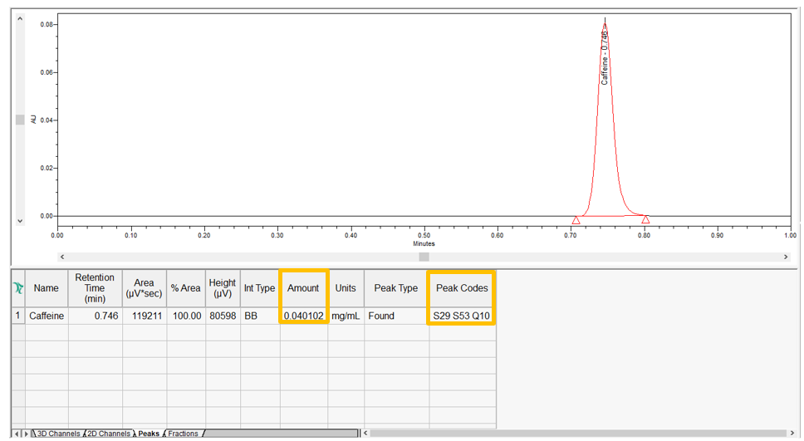
The calculated amount for caffeine is now 0.040102 mg/ml (figure 8).

STEP 9
A stack plot of the three calibration curves and the associated calibration fields appear (figure 9).

STEP 10
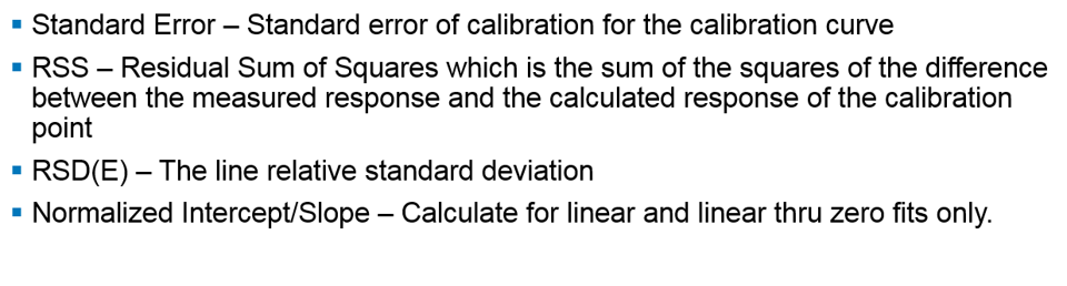
Definitions for some of the calibration fields appear (figure 10).

ADDITIONAL INFORMATION

Final Note: This can be done with either the Pro or QuickStart interface.