What does gradient curve 11 do in Empower 3 - WKB3489

ENVIRONMENT

• Empower 3 Feature release 3

ANSWER

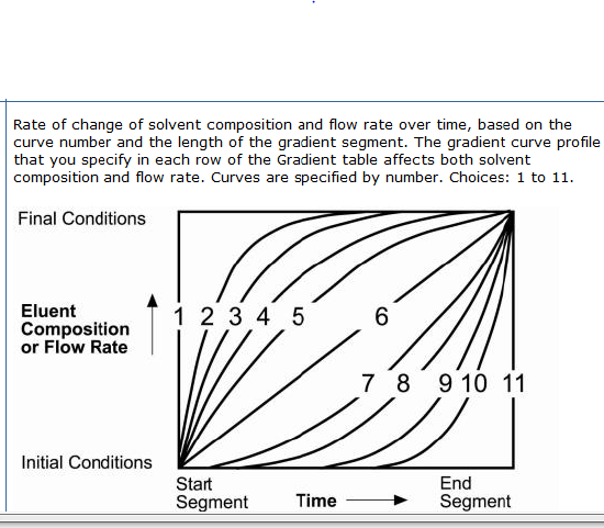
See diagram of curve profiles below.

ADDITIONAL INFORMATION

In Empower,  go to Help Topics > Creating an Instrument Method. Scroll down to see the gradient curve diagram.

There are 11 gradient curves (1-11), which are :
 I.)The step functions:    Curves 1 and 11 
II.)The convex curve set:    Curves 2,3,4,5 
III.)The concave curve set:    Curves 6,7,8,9,10 (includes linear) 

The following variable names will be used throughout: Ti gradient segment start time Tf gradient segment end time t instantaneous run time (chromatography run time) C(t) instantaneous composition at time ‘t’ Ci composition at beginning of segment Cf composition at end of segment N exponent term X defined for each case Gradients are computed over the interval of a ‘segment’, where a single segment may constitute the entire chromatography run, or may be one of several ‘segments’ which are concatenated in order to produce the composition (or flow) profile of the run. In either case, any valid run time ‘t’ will reside in the context of a single segment, and that segment is further characterized by having a start time, an end time (or stop time), an initial condition with respect to composition (or flow), and a final condition with respect to composition (or flow). The variable nomenclature identified above follows from that model of elution control. The step functions are handled as definitions (ie. They do not require continuous evaluation throughout the segment, as the other curve types do). They are defined as: Curve 1: Step immediately to final conditions at segment start time (ie. At Ti, go to Cf) Curve 11: Step to final conditions at segment end time (ie. At Tf, go to Cf) The convex curve set conforms to the following: C(t) = Cf – [ (Cf – Ci) * (X^N) ] Where X = (Tf – t) / (Tf – Ti), and where the notation X^N indicates the quantity X raised to the Nth power, where Curve 2 N = 8 Curve 3 N = 5 Curve 4 N = 3 Curve 5 N = 2 The concave curve set (including linear) conforms to the following: C(t) = Ci + [ (Cf – Ci) * (X^N) ] Where X = (t – Ti) / (Tf – Ti), and where the notation X^N indicates the quantity X raised to the Nth power, where Curve 6 N = 1 Curve 7 N = 2 Curve 8 N = 3 Curve 9 N = 5 Curve 10 N = 8